Have you ever wished your Excel spreadsheets could be more visually appealing and easier to navigate? Imagine if you could add a pop of color to your data validation lists, making your spreadsheets more engaging and impactful. You can! This guide will walk you through the steps of creating a drop-down list in Excel with color, transforming your spreadsheets from plain to polished.

Image: www.vrogue.co
We’ll dive deep into the world of data validation, exploring the power of conditional formatting and its ability to transform your spreadsheets into dynamic and visually appealing platforms. Whether you’re a seasoned Excel expert or a curious beginner, this guide will empower you to create visually stunning and user-friendly spreadsheets that truly stand out.
Understanding the Basics: Data Validation and Conditional Formatting
Before we unleash the power of color, let’s grasp the fundamental concepts: data validation and conditional formatting. Data validation is like a superpower for Excel users, allowing you to control the type of data entered into specific cells. Imagine a scenario where you need a list of fruits to appear in a particular cell. Data validation comes to the rescue, ensuring that only pre-defined fruit options are selected.
Conditional formatting, on the other hand, adds a touch of flair to your cells. It changes the appearance of cells based on specific criteria. Imagine turning a cell green if the value is above a certain target, red if it’s below, or keeping it blue if it’s within the acceptable range. This dynamic color-coding makes complex data instantly interpretable.
Creating Your Colorful Drop-Down List
Now, let’s put these tools to work and create a drop-down list that’s as visually appealing as it is practical. The key is to cleverly combine data validation and conditional formatting. Follow these simple steps:
-
Define Your Data List: Start by creating a list of your desired items. Let’s say you want a list of colors for a design project:
- Blue
- Green
- Yellow
- Red
- Orange
-
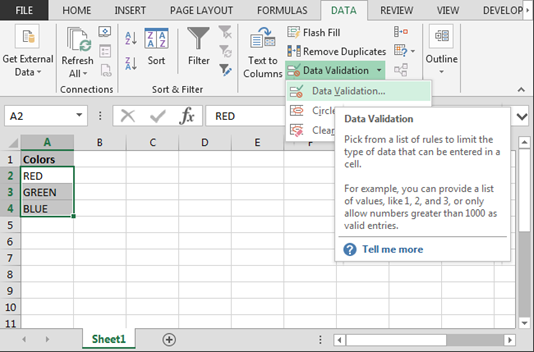
Setting Up the Drop-Down: Select the cell where you want the drop-down list to appear. Go to the Data tab and click Data Validation.
-
Data Validation Rules: In the Settings section, choose List from the Allow dropdown menu. Then, click the Source button and select the range containing your data list (in our example, the color list). Click OK.
-
Conditional Formatting Magic: Now, select the Home tab and click Conditional Formatting. Choose New Rule from the dropdown menu.
-
Applying the Color: In the New Formatting Rule dialog box, select Format only cells that contain and choose Specific text. Enter the first color from your list (Blue) in the “Equals” box. Click Format and select the Fill tab. Choose the color blue and click OK.
-
Creating a Rainbow: Repeat steps 4 and 5 for each color in your list, ensuring the specific text matches the corresponding color in your formatting rule.
Adding More Visual Appeal: Mastering the Art of Conditional Formatting
Once you’ve created your color-coded drop-down list, you can add even more visual impact by applying conditional formatting to the data validation cell itself. This ensures that the cell reflects the chosen color, further enhancing readability.
-
Conditional Formatting Rules: Select your data validation cell. Under Conditional Formatting, choose New Rule.
-
Cell Value Based Rules: Select the Format only cells that contain option and choose Specific Text.
-
Dynamic Color Matching: Enter the color from the first drop-down option (“Blue”) in the “Equals” box. Click Format, select the Fill tab, and choose the blue color.
-
Repeat for Each Color: Repeat steps 2 and 3 for each color in your list, ensuring the cell’s color dynamically changes based on the selected option. This adds a seamless and visually appealing touch to your spreadsheet.

Image: www.vrogue.co
How To Make Drop Down List In Excel With Color
Expert Tips for Creating a Beautiful and Functional Drop-Down List
Crafting a visually appealing drop-down list goes beyond just adding color. Here are some expert tips:
-
Choose Colors Carefully: Use a color palette that’s harmonious and easy on the eyes. Avoid overly bright or clashing colors that might strain user vision.
-
Prioritize Contrast: Ensure sufficient contrast between the font color and background color for accessibility and readability.
-
Keep Formatting Consistent: Maintain consistency in your formatting rules across your spreadsheet.
-
Test Your Work: Thoroughly test your drop-down list functionality to ensure accuracy and eliminate any potential errors.
-
Think About User Experience: Consider your audience’s needs when designing your drop-down list. Choose colors and formats that are user-friendly and intuitive.
Conclusion
Creating a drop-down list with color in Excel might seem like a small step, but its impact on data presentation and user experience is significant. By combining data validation and conditional formatting, you can transform your spreadsheets into visually appealing and insightful tools. Remember, color isn’t just about aesthetics; it’s about making your data more accessible, engaging, and impactful. So, unleash your creativity and start crafting spreadsheets that truly stand out!


