
Have you ever found yourself staring at a massive spreadsheet, overwhelmed by the sheer mass of data? The task of organizing and analyzing it seems daunting. But what if, with just a few clicks, you could visually break up the information, making it easier to parse? Color coding, specifically alternating row colors, can be your secret weapon for transforming your data jungle into a well-organized garden. This article is your guide to mastering the art of color-coding in Excel.

Image: www.educba.com
From simple spreadsheets to complex data analysis, using color coding can enhance your overall experience with Excel. Not only does it make your spreadsheets visually appealing, but it also helps you organize, analyze, and interpret your data more efficiently. Whether you’re a beginner or seasoned Excel user, learning how to color every other row is a valuable skill that can dramatically improve your productivity.
Understanding the Power of Color Coding
Visual Organization:
Imagine navigating a library without any clear shelving or labels. That’s what a spreadsheet without color coding can feel like. Alternating row colors create distinct visual boundaries, making it easier to locate specific data points and follow the flow of information. It’s like having color-coded folders – you can instantly tell which row is related to what, improving your ability to find what you need quickly.
Enhanced Data Analysis:
Think about a complex graph. A few strategically-placed color accents can highlight key trends. Similarly, with color-coded rows, you can easily identify patterns, variations, and outliers in your data. This is especially helpful when working with large datasets. Imagine analyzing sales figures – a quick glance at a color-coded spreadsheet could reveal seasonal trends or product popularity.
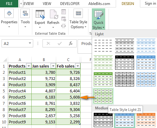
Image: www.coldfrontservices.com
Improved Collaboration:
Sharing a spreadsheet with colleagues becomes infinitely smoother when it’s well formatted. Color-coded rows convey clear and concise information, enabling everyone to grasp the data structure instantly. Think of it like presenting a visually appealing infographic – it engages the audience and facilitates shared understanding.
Different Approaches to Coloring Your Spreadsheet
1. The Manual Method:
This is the classic approach, perfect for smaller spreadsheets where you want complete control over the color choices. Here’s how it works:
- Select the first row: Click on the row number (e.g., 1) to highlight the entire row.
- Apply your desired color: Use the “Fill Color” option from the “Home” tab or the “Font Color” option from the “Font” group. Select your color and click “OK”.
- Select the next row you want to color: Click on the next odd-numbered row (e.g., 3).
- Repeat for all desired rows: Continue selecting every other row and applying your chosen color until you’ve reached the end of your data.
2. Using Conditional Formatting:
This method is ideal for larger spreadsheets and those where you might want to change the coloring scheme later. The best part about Conditional Formatting is it automatically adjusts to added or removed rows. Here’s the step-by-step guide:
- Select the entire data range: Click and drag your cursor over all the rows where you want alternating colors.
- Go to the “Home” tab and click on “Conditional Formatting”: Choose “New Rule…”.
- Select “Use a formula to determine which cells to format”: This allows you to specify conditions for coloring based on a formula.
- Enter the following formula: “=MOD(ROW(),2)=0“. This formula checks the row number and applies the formatting if it’s an even number (every other row).
- Click on “Format” and choose your color: Pick your desired color in the “Fill” tab and click “OK”.
- Click “OK” again to confirm the rule: Your spreadsheet will now have alternating colors.
3. The VBA Approach:
For those comfortable with VBA (Visual Basic for Applications), this method offers ultimate flexibility and customization options. Here’s the process:
- Open the Visual Basic Editor: Press “Alt” + “F11” to open VBA.
- Insert a new module: Go to Insert > Module.
- Paste the following macro code:
Sub AlternateRowColor() Dim row As Integer Dim lastRow As Integer ' Determine last row with data in column A lastRow = Cells(Rows.Count, "A").End(xlUp).Row ' Color every other row For row = 1 To lastRow Step 2 Rows(row).Interior.ColorIndex = 6 ' Light blue (adjust color as needed) Next row End Sub - Modify the code: Change the “ColorIndex” value to your desired color. You can find various color codes in the “ColorIndex” property in the VBA editor.
- Run the macro: Press “F5” to run the code. Your spreadsheet will immediately have alternating colors applied!
Beyond the Basics: Advanced Row Formatting Techniques
Now that you’ve mastered the fundamentals, let’s explore more advanced formatting tricks that can level up your spreadsheets:
1. Alternating Colors with Different Patterns:
Want something more nuanced than just solid colors? Consider experimenting with patterns. Instead of just solid fills, use patterns like “Light Down” or “Gray 75%” for a subtle visual contrast. This can create a dynamic and unique look while still maintaining visual organization.
2. Combining Colors with Font Formatting:
Think beyond just row background colors. You can also change font color or bold text on alternating rows. This adds a further layer of distinction, allowing you to highlight key sections of your spreadsheet even more effectively.
3. Conditional Formatting for Specific Data:
Conditional Formatting offers much more than just alternating colors. Use it to highlight specific data points based on conditions. Imagine highlighting all sales figures over a certain threshold or highlighting rows containing a particular product. This can instantly reveal key trends and insights within your data.
4. Using Excel Themes:
Excel comes with pre-defined themes, complete with color schemes for your entire workbook. Explore these themes to see if they fit your styling needs. This can be a quick and easy way to achieve a consistent look and feel for your spreadsheet.
5. Creating Your Own Custom Styles:
Want to truly personalize your spreadsheet? Excel allows you to create custom styles that include specific font formatting, background colors, and even custom borders. You can save these styles and apply them to any other spreadsheet, maintaining consistency across your Excel projects.
The Importance of Accessibility
As you delve into the world of Excel formatting, remember that accessibility is crucial. While color coding can be a fantastic tool, it’s essential to ensure that it doesn’t create a barrier for people with visual impairments.
Here are some accessibility considerations:
- Use high-contrast color schemes: Avoid using colors that are too similar; aim for visually distinct combinations.
- Provide alternative ways to access data: Consider using data tables or charts that rely on more than just color to convey information.
- Test your spreadsheet with screen readers: Ensure that the structure and formatting are accessible to someone using a screen reader.
How To Color Every Other Row In Excel
Conclusion:
Coloring every other row in Excel is a simple yet powerful technique that can transform your data into a visually appealing and organized masterpiece. From manual selection to the automation of Conditional Formatting and VBA, there are numerous ways to achieve this. By leveraging these techniques, you can enhance your spreadsheet’s clarity, facilitate data analysis, and improve collaboration with colleagues. So, put on your creative hat and explore the vast world of Excel formatting – you’ll be amazed at how these simple techniques can make your data shine.


